AggV3 Principal Components, genetically inferred ancestry and relatedness
We calculated pairwise genetic relatedness amongst samples, inferred genetic ancestry using 1000 Genomes Project's reference populations, and generated universal and superpopulation-specific Principal Components (PCs), using the binary PLINK files derived from the multi-sample VCFs from AggV3. Results from these analyses can be found in CloudOS in the following directory (in File Explorer it is placed under GEL Germline DRAGEN 3.7.8) :
s3://357851407625-germline-aggregate-v3-supporting-data/population-structure-and-relatedness_2026_03_27/
High confidence independent SNPs
The current release of this data is based on 63,523 high-confidence, independent SNPs (referred to as HQ SNPs) generated during the AggV2 release. The detailed description of the selection process of these SNPs is available in the AggV2 documentation, but briefly, these SNPs meet the following criteria:
- Autosomal and bi-allelic,
- Common (MAF>5%) in AggV2 and 1000 Genomes Project Phase 3 data,
- Missingness < 1%
- Median GQ ≥ 30
- Median Depth ≥ 30
- AB Ratio ≥ 0.9
- Completeness ≥ 0.9
- Exclude variants in complex regions, as defined in the 'high LD exclusion regions' file
- Remove all SNPs where the ref/alt combination was AT or GC (A/T, T/A, G/C, C/G), to avoid ambiguous allele swaps
- LD prune using plink version v1.9 with an r2 0.1, 500kb window
- Remove all SNPs which are out of Hardy Weinberg Equilibrium (HWE) in any of the afr, eas, eur or sas super-populations, with a p-value cutoff of pHWE < 1e-5
The AggV2 HQ SNPs were subset from AggV3's PLINK files, and additionally filtered for:
- Missingness < 1%
- Median GQ ≥ 30
- AB Ratio ≥ 0.9
- Not being covered by DUST (low complexity regions)
Note: 5390 out of 63,523 AggV2 HQSNPs were identified as multiallelic in AggV3. Several of them failed on DUST filtering, and 4509 of remaining sites had very low AC values for the secondary allele (AC<5). We therefore included the main alleles (i.e. the ones included in the AggV2 HQ SNPs list) of these new multiallelic sites to preserve the highest possible number of the original HQSNPs, as long as they satisfied the other filtering conditions.
This resulted in a set of 58,763 of HQ SNPs. The PLINK2 file set containing the genotypes of all AggV3 samples at all HQ SNPs can be found here:
| File name | File description |
|---|---|
merge_plink_files.pgen/pvar/psam |
PLINK2 file set containing the genotypes at HQ SNPs of all AggV3 samples. The list of HQ SNPs is available in the .pvar file. |
Genetic relatedness inference
Using these SNPs, we generated a pairwise kinship matrix using the PLINK2 implementation of the KING-Robust algorithm.
These were then partitioned into related (up to, and including third degree relationships) and unrelated sample lists using the PLINK2 --king-cutoff relationship-pruning algorithm, with a threshold of 0.0442.
| File name | File description |
|---|---|
make_king_table.kin0 |
Kinship coefficients in KING table for pairwise relationships with kinship coefficient ≥ 0.0442. |
assign_relatedness.king.cutoff.in.id |
List of unrelated individuals. |
assign_relatedness.king.cutoff.out.id |
List of related individuals. |
make_king_triangle.king.bin |
Full kinship matrix of all AggV3 pairs in PLINK triangular binary format. |
make_king_triangle.king.id |
Sample IDs accompanying the KING triangle. |
{FILE_PREFIX}.log |
PLINK2 run log recording parameters used, sample/variant counts after filtering, and any warnings or errors encountered during execution. E.g. assign_relatedness.log |
Genetic ancestry inference
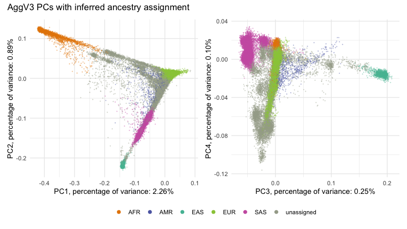
Using PLINK2 binary files from AggV3, we have inferred genetic ancestries using 1000 Genomes Project's data. We used the five broad super-populations, and for more granular results, the 26 populations. Below are the reference tables for populations and super-populations:
| Code | Description |
|---|---|
| AFR | African |
| AMR | Admixed American |
| EAS | East Asian |
| EUR | European |
| SAS | South Asian |
Granular population table
| Population | Population Code | Super Population |
|---|---|---|
| Han Chinese in Beijing, China | CHB | EAS |
| Japanese in Tokyo, Japan | JPT | EAS |
| Southern Han Chinese | CHS | EAS |
| Chinese Dai in Xishuangbanna, China | CDX | EAS |
| Kinh in Ho Chi Minh City, Vietnam | KHV | EAS |
| Utah Residents (CEPH) with Northern and Western European Ancestry | CEU | EUR |
| Toscani in Italia | TSI | EUR |
| Finnish in Finland | FIN | EUR |
| British in England and Scotland | GBR | EUR |
| Iberian Population in Spain | IBS | EUR |
| Yoruba in Ibadan, Nigeria | YRI | AFR |
| Luhya in Webuye, Kenya | LWK | AFR |
| Gambian in Western Divisions in the Gambia | GWD | AFR |
| Mende in Sierra Leone | MSL | AFR |
| Esan in Nigeria | ESN | AFR |
| Americans of African Ancestry in SW USA | ASW | AFR |
| African Caribbeans in Barbados | ACB | AFR |
| Mexican Ancestry from Los Angeles USA | MXL | AMR |
| Puerto Ricans from Puerto Rico | PUR | AMR |
| Colombians from Medellin, Colombia | CLM | AMR |
| Peruvians from Lima, Peru | PEL | AMR |
| Gujarati Indian from Houston, Texas | GIH | SAS |
| Punjabi from Lahore, Pakistan | PJL | SAS |
| Bengali from Bangladesh | BEB | SAS |
| Sri Lankan Tamil from the UK | STU | SAS |
| Indian Telugu from the UK | ITU | SAS |
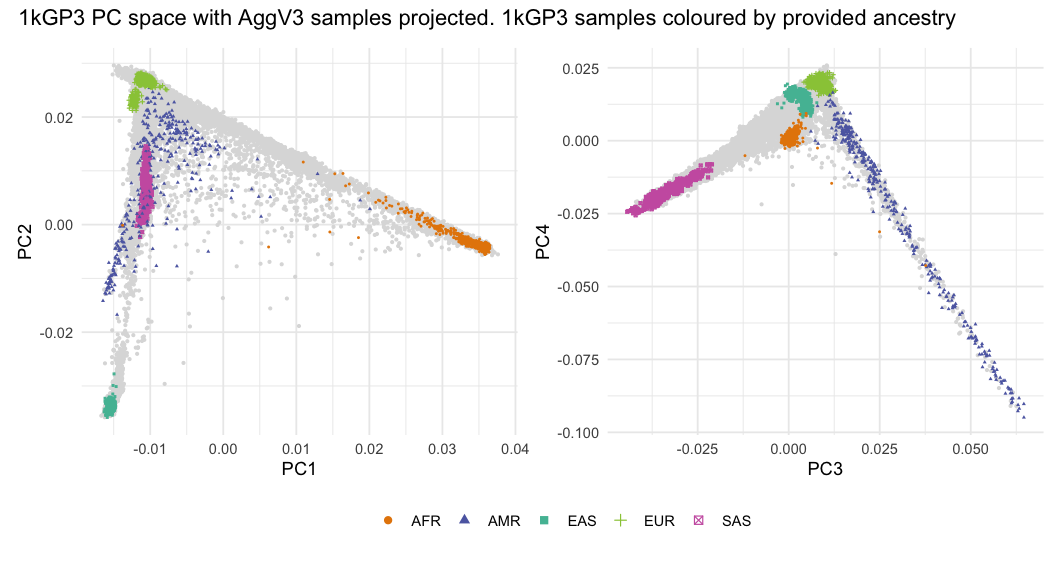
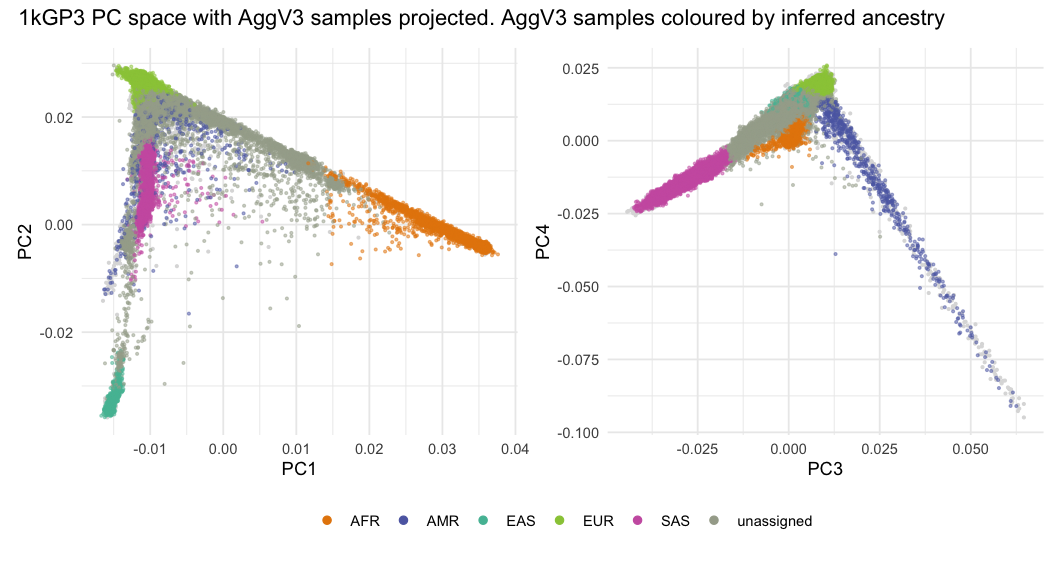
In this release, we used the samples and their population labels from 1000 Genomes Project in a process nearly identical to the one described in AggV2. It is based on PCA, which generates eigenvectors representing the genetic variation among participants as a continuous, multidimensional distribution, in which those with ancestors from the same geographical area often cluster together. Projecting the AggV3 samples onto the 1000 Genomes Project PC space allows us to estimate their genetic ancestries. The process is briefly outlined below:
- We took all unrelated samples from the 1000 Genomes Project.
- Subsetted 1KGP SNPs to just our 58,763 AggV2-derived HQ SNPs (as described above)
- We calculated the first 20 PCs using PLINK2
- We projected the AggV3 data onto the 1000 Genomes Project PC loadings
- We trained a random forest model to predict ancestries based on:
- We trained a random forest model to predict ancestries based on:
a. The first 10 PCs for superpopulations, or 20 PCs for more granular populations
b. Ntrees set to 500
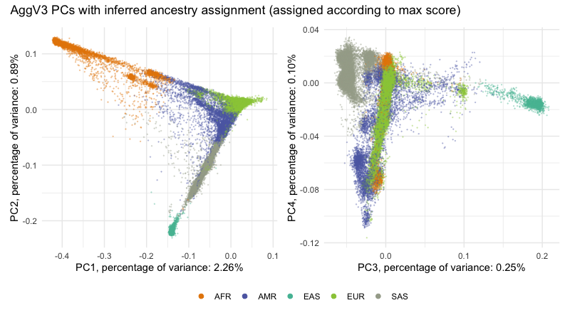
c. 1000 Genomes Project super-population and population labels - Samples with prediction higher than 0.8 was assigned to the assigned ancestry, otherwise it was left as "unassigned"
| File name | File description |
|---|---|
assign_ancestry.predanc |
A TSV file containing the sample_id and ancestry probabilities for each superpopulation (columns 2–6) and population (columns 7–32). The ancestry column indicates the superpopulation for which the sample has a probability > 0.8. |
{ANCESTRY}.txt |
Sample lists for each superpopulation (e.g. EUR.txt). |
Additional ancestry-related resources:
| File name | File description |
|---|---|
project_aggv3_samples_onto_1kgp_pcs.sscore |
Projected PC scores for all AggV3 samples in the 1kGP3 PC space. Each row is a sample; columns are #FID, IID, ALLELE_CT, NAMED_ALLELE_DOSAGE_SUM, and PC1–PC20. |
calculate_1kgp_pcs.acount |
Allele counts for each HQ SNP from unrelated 1kGP samples, generated using --freq counts. Contains chromosome, reference/alternate alleles, and allele counts used as input frequency data for PC projection. |
calculate_1kgp_pcs.eigenvec |
Principal component scores (eigenvectors) for each unrelated 1kGP individual. Each row is a sample; columns are PC1–PCn as specified by --pca. |
calculate_1kgp_pcs.eigenvec.allele |
Allele-specific eigenvector weights for each variant contributing to each PC, produced using the allele-wts modifier. Contains chromosome, ref, and alt columns followed by per-PC loading weights. Used as --score input to project additional samples. |
calculate_1kgp_pcs.eigenval |
Eigenvalues corresponding to each principal component. |
{FILE_PREFIX}.log |
PLINK2 run log recording parameters used, sample and variant counts after filtering, and any warnings or errors encountered during execution. |
Ancestry summary stats
| Population | N | % |
|---|---|---|
| AFR | 361 | 32.61 |
| AMR | 624 | 0.45 |
| EAS | 1199 | 0.87 |
| EUR | 10956 | 79.16 |
| SAS | 1273 | 9.20 |
| unassigned | 1067 | 27.71 |
Principal Components
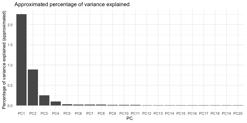
We ran PCA as implemented in PLINK2 using 58,763 HQ SNPs. We calculated 50 PCs on 102,341 unrelated individuals. Due to the high number of samples, we used the -approx modifier in the PLINK command. We then projected all 138,406 individuals (related and unrelated) onto these PCs with PLINK2's -sscore functionality with variance standardisation, computed without mean imputation for missing genotypes.
We also provide the first 50 PCs calculated on samples from each super-population, using the inferred genetic ancestries described above. We ran PCA as described above on unrelated sets of individuals from each super-population, and then projected all individuals onto these PCs.
| File name | File description |
|---|---|
project_aggv3_samples_onto_unrelated_aggv3_pcs_{ANCESTRY}.sscore |
Projected PC scores for each sample in the ancestry‑filtered set. ALL refers to all AggV3 samples. Each row is a sample; columns are #FID, IID, ALLELE_CT, NAMED_ALLELE_DOSAGE_SUM, and PC1–PC50. |
calculate_unrelated_aggv3_pcs_{ANCESTRY}.acount |
Allele counts for each variant in the ancestry‑filtered sample subset, generated using --freq counts. Contains chromosome, reference/alternate alleles, and allele counts used as input frequency data for PC projection. |
calculate_unrelated_aggv3_pcs_{ANCESTRY}.eigenvec |
Principal component scores (eigenvectors) for each unrelated individual in the ancestry‑filtered set. Each row is a sample; columns are PC1–PCn as specified by --pca. |
calculate_unrelated_aggv3_pcs_{ANCESTRY}.eigenvec.allele |
Allele‑specific eigenvector weights for each variant contributing to each PC, produced using the allele-wts modifier. Contains chromosome, ref, and alt columns followed by per‑PC loading weights. Used as --score input to project additional samples. |
calculate_unrelated_aggv3_pcs_{ANCESTRY}.eigenval |
Eigenvalues corresponding to each principal component. |
{FILE_PREFIX}.log |
PLINK2 run log recording parameters used, sample and variant counts after filtering, and any warnings or errors encountered during execution. |
Note on monomorphic SNPs
During the PCA projection step, we found that 154 SNPs in the EAS population were monomorphic in the unrelated set.
Due to the variance-standardise option used in PLINK, we removed these SNPs from the EAS projection step to complete the projection.
Monomorphic SNPs were identified by filtering the .acount files per superpopulation for sites where AF = 0 or AF = 1.
We acknowledge that Hardy–Weinberg Equilibrium filtering should have removed these sites and accept this as a caveat of using the HQ SNPs derived in AggV2.
We intend to correct this in future releases.
The list of monomorphic SNPs provided in the main output directory:
| File name | File description |
|---|---|
identify_monomoprhic_snps_{ANCESTRY}.txt |
A list of monomorphic SNPs. Files are empty for all populations except EAS. |
AggV3 PC plots
Below we show the first 4 PCs, derived from PCA on the AggV3 samples. The graphs show samples coloured by their inferred genetic ancestry (using a threshold of T=0.8), and 'best-guess' ancestry based on their inferred super-population. Additionally, we provide the percentage of variance explained by each principal component, estimated by dividing the eigenvalues by the total number of samples used to calculate the PCs.