AggV2 ancestry inference¶

Using the multi-sample VCFs from aggV2, we have estimated probabilities of genetic ancestry for five broad super-populations, calculated Principal Components (PCs) for participants in aggV2, and calculated pairwise relatedness amongst samples. Alternatively, we have also calculated more fine-grained mappings to 15 worldwide reference populations for AggV2.

We estimated broad genetic ancestry using super-populations from the 1000 genomes project phase 3 (1KGP3) as the truth, by generating PCs for 1KGP3 samples and projecting all aggV2 participants onto these. The five broad super-populations are:

Code	Description
`afr`	African
`amr`	Admixed American
`eas`	East Asian
`eur`	European
`sas`	South Asian

Ancestry inference¶

We used the 1KGP3 to infer ancestry as follows:

We took all unrelated samples from the 1KGP3
We subsetted to just our 188382 HQ SNPs
Further filtered for MAF > 0.05 in 1KGP3 (as well as in our data)
We calculated the first 20 PCs using GCTA
We projected the AggV2 data onto the 1KGP3 PC loadings
We trained a random forest model to predict ancestries based on
1. First eight 1KGP3 PCs
2. set Ntrees = 300
3. Train and predict on 1KGP3 amr, afr, eas, eur and sas super-populations

Model performance¶

Below we show the summary data for the random forest model fit. The out-of-bag (OOB) error rate and confusion matrix show very high performance in the prediction of 1KGP3 super-populations.

Random Forest ancestry model fit

Call:
 randomForest(x = rfdat[, pcs1_8], y = SuperPopLabels, ntree = 400,      keep.inbag = T)
               Type of random forest: classification
                     Number of trees: 400
No. of variables tried at each split: 2

        OOB estimate of  error rate: 0.24%
Confusion matrix:
    AFR AMR EAS EUR SAS class.error
AFR 638   2   0   0   0  0.00312500
AMR   3 342   0   1   0  0.01156069
EAS   0   0 498   0   0  0.00000000
EUR   0   0   0 499   0  0.00000000
SAS   0   0   0   0 480  0.00000000

The probabilities for each individual is found at:

/gel_data_resources/main_programme/aggregation/aggregate_gVCF_strelka/aggV2/additional_data/ancestry/MAF5_superPop_predicted_ancestries.tsv

If you are interested in more fine-grained population structure, we provide a set of ancestry predictions based sub-population ancestries from the 1KGP3. The steps to calculate are as above and differ only for steps 3 and 6.

3 - MAF filter of >0.01 for 1KGP3 and aggV2 data

6 - We trained a random forest model to predict ancestries based on 1KGP3 sub-populations

These data are available at:

/gel_data_resources/main_programme/aggregation/aggregate_gVCF_strelka/aggV2/additional_data/ancestry/MAF1_subpops/MAF1_subPop_predicted_ancestries.tsv

Ancestry summary stats¶

Below is a summary table for the number of individuals (and as a percent of the cohort) assigned with a probability of >0.8 for any one ancestry.

Population	N	%
`afr`	2002	2.56
`amr`	238	0.3
`eas`	518	0.66
`eur`	62349	79.7
`sas`	7195	9.2
unassigned	5893	7.54

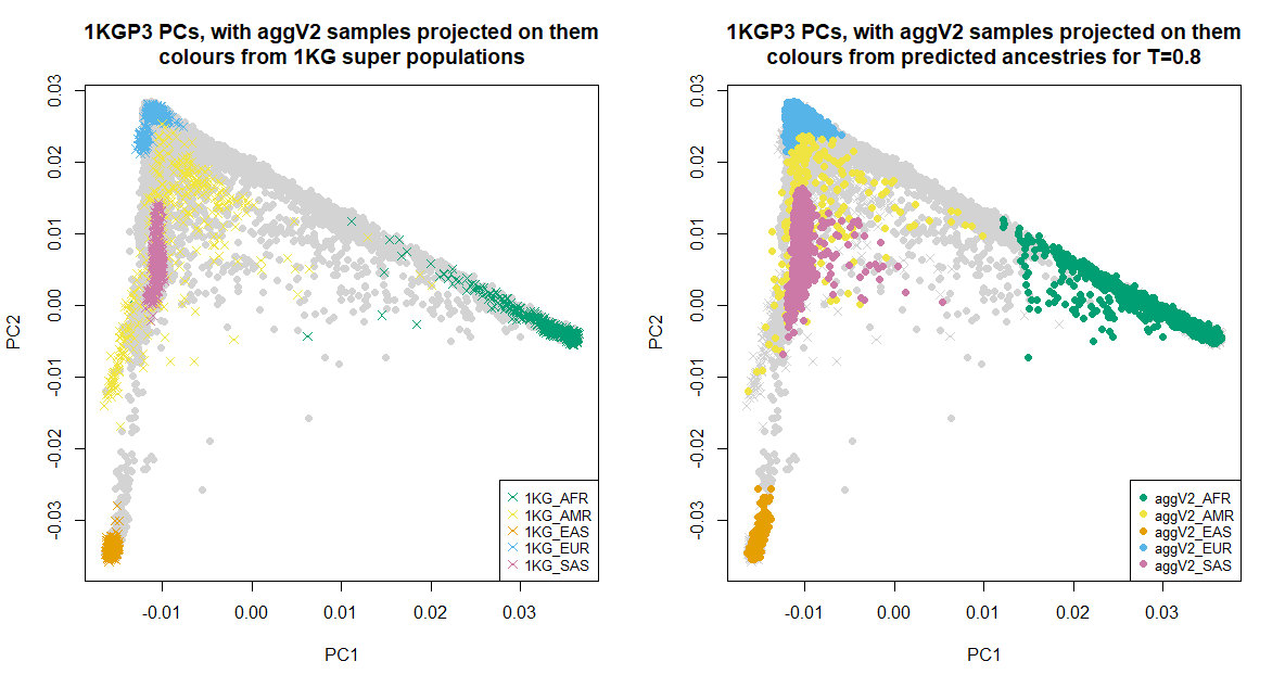
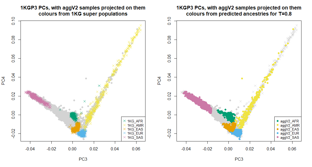
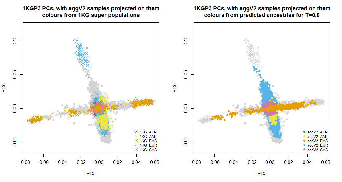
PCs with 1KG samples and projected aggV2 samples, coloured by predicted ancestry¶

Below we show the first six PCs, which were used for the ancestry inference of the aggV2 samples. The plots to the left show all samples (in grey), with the 1KGP3 samples plotted in different colours by super-population. The plots to the right show all samples (in grey), with the aggV2 samples plotted in different colours by predicted super-population (using a threshold of T = 0.8). 1KG samples are represented by crosses, and aggV2 samples by solid circles.

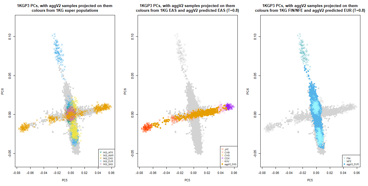
The following plot focuses on EUR and EAS sub-populations from 1KGP3. 1KG samples are represented by crosses, and aggV2 samples by solid circles. PCs for all 1KGP3 and aggV2 samples are included, in grey. In addition:

Left: 1KGP3 samples in different colours by super-population

Middle: 1KGP3 samples in different colours by EAS sub-populations, with aggV2 predicted EAS plotted on top

Right: 1KGP3 samples in different colours by NFE and FIN populations, with aggV2 predicted EUR samples plotted in darkblue.