The GWAS pipeline
This pipeline allows you to run Genome Wide Association analyses on Genomics England data. After building a cohort (either a case-control cohort for binary phenotypes or a scored cohort for continuous phenotypes), you can run this workflow to identify variants that are enriched for the phenotype.
Licensing
This pipeline has been released under the MIT license.
Output from this pipeline will be subject to review by the Airlock committee. You will need to ensure that you are familiar with Airlock procedures and review the data that is submitted for export to ensure that it complies with the procedures and expectations stated in the user guide.
Introduction
To accommodate GWAS at a large scale, we have developed a pipeline based on workflow language Nextflow.
Given the phenotype file and some additional arguments as input, the pipeline performs several steps of appropriate site Quality Control (QC) on high-coverage whole genome data and then runs mixed model association analysis.
Running the pipeline
To run the GWAS pipeline, you need to run the following steps:
- Build a case/control cohort
- Create a phenofile of the cohort
- Create a list of genomic files to run the GWAS on
- Create further input files
- Launch the pipeline as an interactive job
- Monitor the jobs
- View the output
- Export the results
GWAS models
Different GWAS methods are available for different types of analysis. The pipeline supports binary, continuous and time-to-event phenotypes. All methods are state-of-the-art, are based on similar method principles and are expected to produce similar outputs. Choose the method that best suits your cohort and phenotype of interest.
These methods are available
- SAIGE: For binary of continuous phenotypes. By default, the pipeline uses SAIGE as we have used it extensively as part of our work with international consortia.
- GCTA fastGWA: For binary or continuous phenotypes. GCTA fastGWA, is included because it has been shown to be several-fold faster than SAIGE.
- GATE: for time-to-event phenotypes. GATE is the only existing and scalable approach for mixed model analysis of time-to-event phenotypes.
Build a case/control cohort
You can build your cohort by your preferred method. We provide some tutorials on building cohorts using our Labkey API.
Create a phenofile of the cohort
The phenofile is the required input for the GWAS pipeline.
This is a space- or tab-separated text file that contains the sample information. The file must have a header as this will be used to specify the columns to use in your command.
The phenoFile must include a minimum of three columns: sample ID, sex specification and phenotype specification. It can optionally also include other columns to specify other covariates, such as age and principal components.
-
Sample ID column: The pipeline will read the sample ID from the column specified with option
--sampleIDcol. If you're running the pipeline on Genomics England data, the sample ID should be the platekey ID because this is what is specified in the aggregate genomic data. For other data, you can use whatever ID is appropriate for that data -
Sex specification column: The pipeline will read the sex info from the column specified with option
--sexCol. Males must be specified as 0 and females as 1. -
Phenotype specification column: The pipeline will read the phenotype from the column specified with option
--phenoCol(see below)
For a binary phenotype, use 0 for controls and 1 for cases:
For continuous phenotypes, this should be score or value of the phenotype:
For time-to-event traits you have to specify the censoring information as follows:
1: individual experienced the event during the study period.
0: individual is censored (i.e., did not experience the event during the study period).
This info is read from the column specified with option --phenoCol.
In this case you also must add the option --eventTimeCol to specify the column containing the time variable.
Create a list of genomic files to run the GWAS on
The pipeline required a list of genomic files, these can be either VCF or bgen or pgen format.
List requirements:
- The list must contain comma-separated file locations
- The files must exist and not be empty.
- Specify chromosomes with "chr" prefix, i.e., "chr1" rather than "1" and chromosome X should always be specified as "chrX".
A list of vcf files that contain the genotype data that will be used in the GWAS.
The list is comma-separated, expects a header and has three fields: chr, vcf, index.
Example of a vcflist:
The pipeline will loop over each file on the list in a parallel fashion creating "channels" of data that pass from one process to the next (e.g, masking → siteQC → SAIGE association analysis).
For example, if the genetic data is split by chromosome, then it will have 22 (autosomes) + 1 (chrX) = 23 channels.
The data could be split further, for example each chromosome could be split into several chunks, thus having thousands of channels processing in parallel massive amounts of data.
A list of bgen files that contain the genotype data that will be used in the GWAS.
The list is comma-separated, expects a header and has four fields: chr, bgen, index, samplefile
Example of a bgenlist:
Example of creating a bgen list
Here is an example bash script. It can be modified to build any type of list for .bgen files that are split by chunk or by chromosome. Similar logic can be followed for --vcflist and --pgenlist arguments for analysis of VCF and pgen files, respectively.
This example builds the list based on genomic files that contain aggV2 data that has been filtered for PASS sites with MAF>0.1%.
You can modify this script to build any type of list for .bgen files that are split by chunk or by chromosome.
*Note that for bgenfiles for PASS variants with MAF>0.001, the chunk chr11_51386977_52570776 will not be included in the list as no variants existed for this chunk after applying the filters for this set of files.
Create further input files
You also need an unrelatedfile and a HQplinkfile.
unrelatedFile
This file specifies the set of individuals that are unrelated. It will be used for the HWE test as part of the siteQC procedure.
Genomics England provides this file for a set of unrelated individuals, found at:
/gel_data_resources/main_programme/aggregation/aggregate_gVCF_strelka/aggV2/additional_data/PCs_relatedness/relatedness/GEL_aggV2_MAF5_mp10.king.cutoff.unrelated.id
If you wish to create your own file, the format is what is provided as input to --keep command from plink1.9.
Example unrelated file:
In most cases the two columns will be identical (as family information is not needed).
Use the platekey IDs as these are used in all the aggregate genomic data.
HQplinkfile
This option will designate the plink files identifying high quality independent SNPs. To simplify the process the flag will set a prefix for the files and expand these to cover the suffixes needed. This fileset will be used to construct the GRM and fit the null model when running the mixed model association analysis.
The suffix pattern will be:
.{bed,bim,fam}
This corresponds to the triplet of files that are used by plink.
If you are using the aggregate VCFs, you can use the following file:
/gel_data_resources/main_programme/aggregation/aggregate_gVCF_strelka/aggV2/additional_data/HQ_SNPs/GELautosomes_LD_pruned_1kgp3Intersect_maf0.05_mpv10.{bed,bim,fam}
Launch the pipeline as an interactive job
In the RE you can run the pipeline from its current location in the /pgen_int_data_resources/workflows/BRS_tools_GWAS_nf/v1.3/ directory. In the CloudRE, you can select the pipeline from your workspace tools.
Create a submission script to to launch the pipeline, replacing the dummy example paths shown here with the actual files:
You can now run this with:
bsub < submission_script_filename.sh
Required arguments
To run the job, you require the following arguments:
| Argument | Analysis phenotype | Brief description | Example |
|---|---|---|---|
--phenoFile |
binary/quantitative/time-to-event |
File location of the input file containing phenotypes. | --phenoFile 'example.pheno' |
--unrelatedFile |
binary/quantitative/time-to-event |
File location of the input file with list of unrelated individuals. | --unrelatedFile '/gel_data_resources/main_programme/aggregation/aggregate_gVCF_strelka/aggV2/additional_data/PCs_relatedness/relatedness/GEL_aggV2_MAF5_mp10.king.cutoff.unrelated.id' |
--vcflist, --bgenlist or --pgenlist |
binary/quantitative/time-to-event |
File location of the input file with list of genomic files containing the variants to be tested for association with outcome. | --bgenlist 'example.csv' |
--HQplinkfile |
binary/quantitative/time-to-event |
File location of the input trio of files containing the high-quality independent variants for calculating the GRM. | --HQplinkfile '/gel_data_resources/main_programme/aggregation/aggregate_gVCF_strelka/aggV2/additional_data/HQ_SNPs/GELautosomes_LD_pruned_1kgp3Intersect_maf0.05_mpv10.{bed,bim,fam}' |
--sampleIDCol |
binary/quantitative/time-to-event |
Column name from the phenoFile containing the platekey ID. The sampleIDCol must specify platekey IDs because platekey IDs are used in all the aggregate genomic data. | --sample_IDCol 'platekey' |
--sexCol |
binary/quantitative/time-to-event |
Column name from the phenoFile containing the sex column. Males must be specified as 0 and females as 1. | --sexCol 'sex' |
--phenoCol |
binary/quantitative/time-to-event |
Column name from the phenoFile containing the phenotype column. | --phenoCol 'pheno' |
--eventTimeCol |
time-to-event |
Column name from the phenoFile containing the time variable, if time-to-event analysis is desired. Additional arguments --traitType must be set to 'survival', and --gwasmethod must be set to 'GATE' if this option is specified. |
--eventTimeCol 'time' |
Optional additional arguments
| Argument | Analysis phenotype | Brief description | Example |
|---|---|---|---|
--gwasmethod |
binary/quantitative/time-to-event |
Specify method to run GWAS. Either 'SAIGE', 'GCTA' or 'GATE'. Default is 'SAIGE'. |
--gwasmethod 'SAIGE' |
--traitType |
binary/quantitative/time-to-event |
Specify trait to be analysed. Either 'binary', 'quantitative' or 'survival'. 'survival' works only with 'GATE' method. |
--traitType 'binary' |
--profile |
binary/quantitative/time-to-event |
configuration for HPC cluster ('cluster') or cloud research environments ('cloud') | --profile 'cluster' |
--covariateCols |
binary/quantitative/time-to-event |
Specify columns in the phenoFile to be used as covariates in the regression. | --covariateCols 'age,pc1,pc2' |
View the output
As output, the pipeline produces GWAS summary statistics, manhattan and qqplot figures.
The output folder contains the results of the plotting process: the manhattan plot, ggplot and the GWAS summaries (e.g., beta and P-values) that can be used directly as input for other downstream analyses such as heritability estimation, fine-mapping and TWAS.
Each process emits outputs that are directed to the child processes, until the pipeline finishes. To avoid excessive usage of disk space and duplication, outputs from all other processes are soft-linked from the /work directory.
In all cases, the outputs of this pipeline will be examined case-by-case if they are submitted for export through the Genomics England Airlock process and we provide no guarantees that they will be accepted. In all cases, you have to verify that their submission is compatible with Airlock policies.
Export the results
Results folders can be exported through Airlock, subject to review by the Airlock committee. It is your responsibilty to ensure that your exports comply with the Airlock rules
Tutorial video
Details of the job
Pipeline process overview
The pipeline runs a sequence of processes that are submitted as jobs to the scheduler.
A typical use-case of the workflow consists of the following steps:
1. parse_pheno: Parses the provided --phenoFile to generate inputs for downstream processes.
- gwas_siteQC: Performs site Quality Control.
Filters to keep only sites with minor allele frequency maf>0.5% and low missingness (<2%) and performs a differential missingness test between cases and controls (keeps variants with P>1e-5), and an HWE test on unrelated controls (keeps variants with P>1e-6). For quantitative traits, the differential missingness test is skipped and only HWE is performed on the whole unrelated sample (keeps variants with P>1e-6).
-
gwas_SAIGE_fit_null_glmm, gwas_GCTA_fit_null_glmm or gwas_GATE_fit_null_glmm: Fits the null SAIGE, GCTA or GATE models.
-
gwas_SAIGE_spa_tests_bgen, gwas_GCTA_spa_tests_pgen or gwas_GATE_spa_tests_bgen: Runs association GWAS tests across the genome for SAIGE, GCTA or GATE.
A MAC>20 filter is applied to this process by default for SAIGE (in addition to the gwas_siteQC maf filter). This is because the saddlepoint approximation used in SAIGE for single-variant association tests does not work well for variants with low MAC.
- plotting: Concatenates resulting GWAS summaries and generates manhattan and qqplot.
Plots are rudimentary and y-axis starts from 1e-2 by default, to reduce computation.
Monitor the pipeline
You can examine the progress of the workflow while it is running or after it has completed by checking the file with suffix .trace. Whether to generate this file and its name is controlled by the argument flag -with-trace.
Within this file, you will see details for COMPLETED or FAILED processes, their duration, peak memory and cpu usage.
FAILED jobs/processes will be retried (resubmitted) three times by default.
If lots of jobs fail
If you start seeing many jobs in FAILED status in trace file or if the same job fails consecutively multiple times, its best to manually kill the master job that was used to launch nextflow, investigate why the processes are failing, modify inputs, and then relaunch with identical inputs and option -resume as the example above to resume progress.
To investigate a process/job further, find the hash column for the process/job in the .trace file. The folder containing the output will be under work/ followed by the hash ID.

for example the folder for the first listed process in the figure above will be:
work/56/cc5ebc...
The folder name is actually slightly longer but the hash uniquely identifies the first part of the name of the folder and the rest can be auto-completed by pressing tab.
Within each of these subfolders, .command.out and .command.err files will contain the standard output and error logs which can be examined to find the causes of possible errors. In these subfolders we can also find .command.sh that contains the actual bash command that was run. These files are very useful for adding to issues and tickets when running into errors and FAILED processes/jobs.
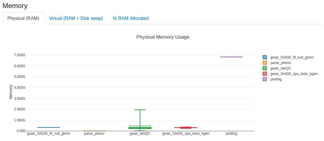
Workflow resource usage
An optional argument you can use is -with-report:
-with-report ${trait}.html
This generates an html report that can be open with a browser like Firefox and display the distribution of allocated resources for processes in terms of CPUs, RAM, time, I/O. An snapshot of RAM usage for a run of the psoriasis is shown below.
Example: performing an analysis on aggV2 for binary psoriasis phenotype
Creation of required input
For the initial phases of the analysis, you will need to prepare two files:
- a phenofile from the cohort of selected participants
- a list of genetic data to parse (this will form the basis of the vcf/bgen files list)
For this example we will be working with BGEN files.
The GWAS pipeline can be run both on the HPC and with CloudOS.
Run on the HPC cluster
Creation of cohort in R and generation of phenoFile
Creation of cohorts for GWAS is typically an involved process where the phenotype definition and the covariates to use has to be carefully thought.
For the purposes of this example we provide R code to demonstrate the generation of a simple case/control phenotype where controls are matched in a 5:1 ratio to cases in respect to sex.
In a real use-case, the following script or derivatives would have to be carefully modified to fit the purposes of each analysis.
As R uses substantial RAM when running the Labkey queries, please make sure to run these while providing enough compute resources, e.g., by launching an interactive session (modify requirements accordingly):
bsub -q inter -P bio -Is -n 1 -R rusage[mem=10000] -M 10000 /bin/bash
Then load the R module:
module load R/4.3.3
Then run R code below to define a psoriasis case cohort with matched on sex 5:1 controls:
Creation of psoriasis cohort, query in RE1 for aggV2 aggregate
Creation of list of genomic files to run GWAS on
We provide here bash scripts to generate the required file for --bgenlist option which specifies the bgen files containing the genomic data that the association analysis will run on.
The script operates on the list of genomic chunks, building line-by-line the file.
It can be modified to build any type of list for .bgen files that are split by chunk or by chromosome. Similar logic can be followed for --vcflist and --pgenlist arguments for analysis of VCF and pgen files, respectively.
In this example we build the list based on genomic files that contain aggV2 data that has been filtered for PASS sites with MAF>0.1%.
However, it can be modified to build any type of list for .bgen files that are split by chunk or by chromosome.
Creation of bgenlist for PASS variants with MAF>0.1%
*Note that for bgenfiles for PASS variants with MAF>0.001, the chunk chr11_51386977_52570776 will not be included in the list as no variants existed for this chunk after applying the filters for this set of files.
Interactive job launch
Then run the Nextflow GWAS pipeline on the psoriasis dataset in a terminal by pasting the code below, which will submit the job to the interactive queue.
You can also submit to 'medium' queue in case you want to run several GWAS jobs. Jobs with default parameters, are unlikely to take more than 24h to complete, but this largely depends on the workload of the cluster which might necessitate using the 'long' queue.
??? example "Submission of gwas for psoriasis to interactive queue of the HPC"

``` bash linenums="1"
trait=psoriasis

echo "
# BSUB -q inter
# BSUB -P <ProjectCode>
# BSUB -o ./logs/%J.stdout
# BSUB -e ./logs/%J.stderr
# BSUB -J ${trait}
# BSUB -n 1
# BSUB -R "rusage[mem=10GB] span[hosts=1]"
# BSUB -cwd .

mkdir -p ./logs
module purge
module load nextflow/22.10.5 singularity/4.1.1

nextflow run /pgen_int_data_resources/workflows/BRS_tools_GWAS_nf/v1.3/main.nf \
-bg -with-trace ${trait}.trace -with-report ${trait}.html -resume -dsl1 \
--phenoFile 'pheno_psoriasis_matched5.tsv' \
--unrelatedFile '/gel_data_resources/main_programme/aggregation/aggregate_gVCF_strelka/aggV2/additional_data/PCs_relatedness/relatedness/GEL_aggV2_MAF5_mp10.king.cutoff.unrelated.id' \
--bgenlist 'gel_mainProgramme_aggV2_filteredPASS_bgenlist.csv' \
--HQplinkfile '/gel_data_resources/main_programme/aggregation/aggregate_gVCF_strelka/aggV2/additional_data/HQ_SNPs/GELautosomes_LD_pruned_1kgp3Intersect_maf0.05_mpv10.{bed,bim,fam}' \
--sampleIDCol 'platekey' \
--sexCol 'sex' \
--phenoCol 'pheno' \
--covariateCols 'sex,pc1,pc2,pc3,pc4,pc5,pc6,pc7,pc8,pc9,pc10' \
--gwasmethod 'SAIGE' \
--profile 'cluster' \
--outdir ${trait} \
--output_tag ${trait} \
--clusterOptions -P <ProjectCode> --\R rusage[mem=<Num>] -M <Num>

" > GWAS_${trait}.sh

bsub < GWAS_${trait}.sh
```
Note the extra --outdir and --output_tag options used here determine the folder name for the pipeline output and the prefix for the final GWAS summary files. If those are omitted, the output will be stored by default in folder 'results' and the prefix for GWAS output files will be 'trait'.
Workflow output folders and files
The folder "psoriasis" (the folder name was specified with argument --outdir) will have the following sub-directories that will be generated as the workflow is running (check here for more output details):
-
error_report: Folder contains text files which record two types of errors: "emptyinput" and "novariantsleft". These two errors do not break the pipeline, processes will still complete when the input genomic VCF/bgen file is empty or when there are no variants left after QC filters, respectively.
-
gwas_bgen_siteQC: Folder contains soft links to work folder for the final QC'd bgen files just before they are passed to the association software.
-
gwas_SAIGE_fit_null_glmm: Folder contains soft links to files from the null fit of SAIGE.
-
gwas_SAIGE_spa_tests: Folder contains soft links to per-chunk/chromosome summary statistic outputs.
-
plotting: Folder contains the concatenated GWAS summaries across all chunks/chromosomes.